| Physics |
| |
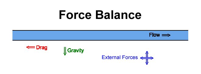
| Force Balance |
| |
 |
| |
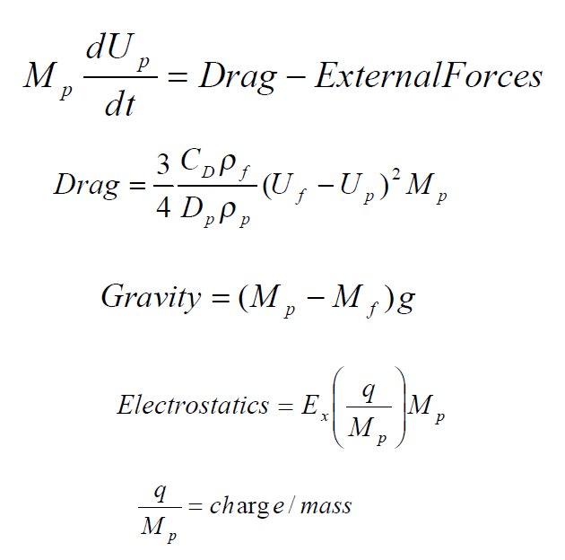
| The force balance with its three forces is written in a differential format.
The drag force uses a drag coefficient which will vary depending on
the fluid and particle velocities. The electrostatic term, while very
important, in some cases is hard to measure and quantify. |
| |
 |
| |
| |
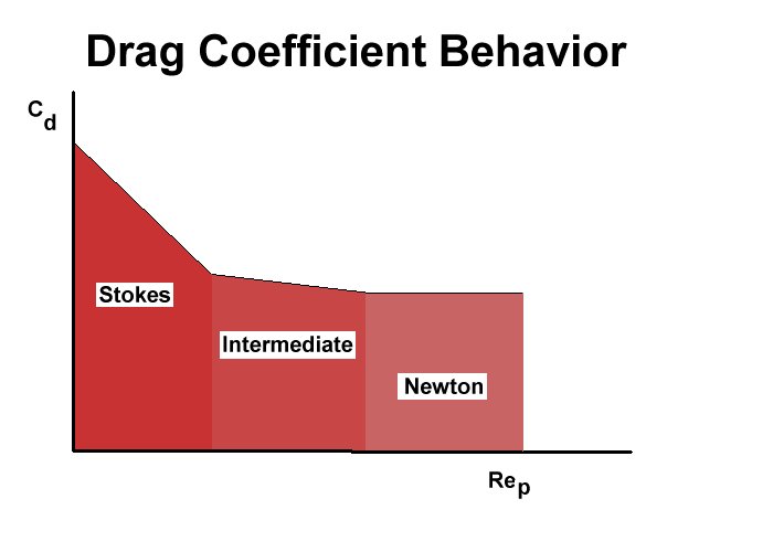
| The drag coefficient can be represented according the flow condition
surrounding the particle. For low flows or relative flows the drag
coefficient can be given with a simple equation that is termed the
Stokes regime. This is often likened to the laminar flow condition.
The intermediate range has an empirical expression for the drag
coefficient and the turbulent flow regime is presented by a constant
drag coefficient of 0.44. This region is called the Newton regime.
|
| |
| General CD Expressions |
| CD = 24/Rep | Rep < 2.0 | Stokes |
| CD = 18.5/Rep0.6 | 0.5 < Rep < 500 | Intermediate |
| CD = 44 | 500 < Rep < 2 x 10³ | Newton |
|
| |
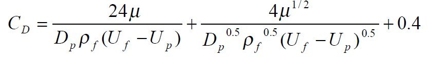
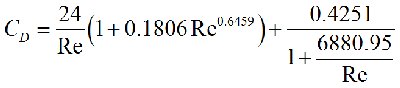
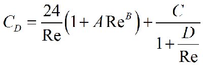
| Kaskas has been able to develop one equation that would serve for all the three flow regimes experienced by the particle. The first term
is essentially the laminar flow or Stokes regime while the second term
brings in the intermediate range and as the velocity increases the drag
coefficient approaches a constant.
|
| |
| Kaskas Coefficient of Drag is defined as: |
| |
 |
| |
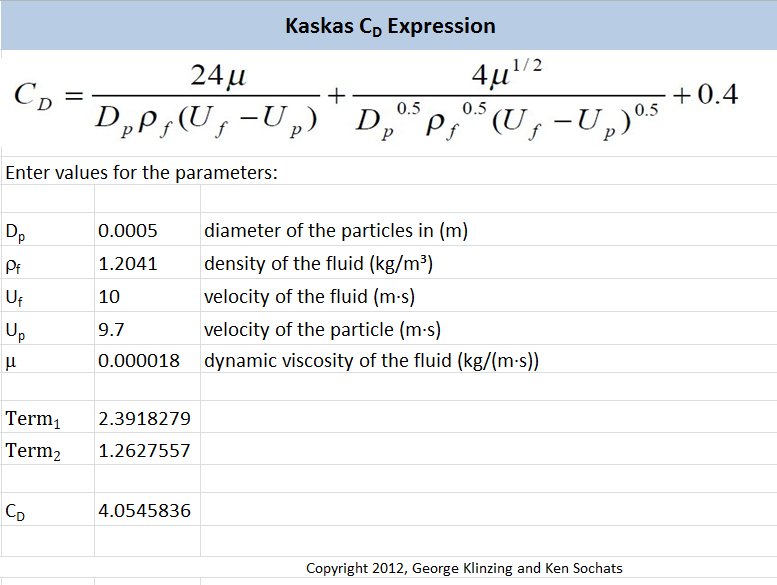
where:
- Dp = diameter of the particle (m)
- ρf = density of the fluid (kg/mł)
- Uf = velocity of the fluid (m·s)
- Up = velocity of the particle (m·s)
- μ = dynamic viscosity of the fluid (kg/(m·s))
- CD = Kaskas coefficient of drag
|
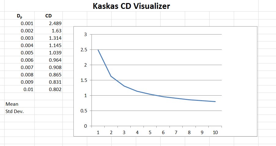
The image below shows a screenshot of a spreadsheet that calculates the Kaskas coefficient of drag.
By clicking on the image you can download the spreadsheet and enter values for yourself. |
| |
 |
| |
| The image below shows a graph of the effect of changing the hydraulic diameter of the pipe (m) in the example above from .001 to .01 in increments of .001 m.
|
| |
 |
| |
| Click on the graph to download a copy of the graphing spreadsheet. Instructions for the spreadsheet program can be found by clicking here. |
| |
| Resources: |
G.E. Klinzing, F. Rizk, R. Marcus and L.S. Leung, Pneumatic Conveying of Solids: A theoretical and practical approach (Particle Technology Series), 3rd ed., Springer, June 22, 2010, ISBN-10: 9048136083, ISBN-13: 978-9048136087.
|
|
| |
|
| |
| In the turbulent flow regime Pettyjohn and Christiansen looked
closely at the drag coefficient and suggest that the sphericity of the
particle is a dominant factor for the drag coefficient. The sphericity
is the degree to which a particle deviates from a true spherical shape.
For a value of the sphericity of 1.0 the particle is a perfect sphere.
|
| |
| The drag coefficient is seen to decrease with the increase in the particle
Reynolds number as shown in the figure.
|
| |
| CD = 5.31 - 4.88 ψ |
| Where ψ is the sphericity of the particle. |
| |
| There are a couple of key notes that are necessary when dealing with the above overall balance. The electrostatic force can be very dominant and is very dependent on the environmental conditions especially the relative humidity. The use of non conducting pipes anywhere in the system can generate tremendous electrostatic forces. A non conducting elbow made of rubbery materials are prime suspects to generate these forces.
Another point is the particle Reynolds number is often used in pneumatic conveying analyses. This number depends on the relative velocity between the fluid and the particle. In addition the length variable is the diameter of the particle.
The tube Reynolds number is based solely on the diameters of the pipe along with the fluid velocity. This employs extensively in single phase flow applications
|
| |
| The drag coefficient is seen to decrease with the increase in the particle
Reynolds number as shown in the figure.
|
| |
 |
| |
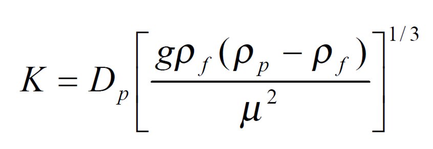
| Another way to determine the proper drag coefficient is to look at a (K)
factor which will give the specific ranges of applicability – Stokes
– Intermediate - Newton
|
| |
 |
| |
K < 3.3 Stokes
3.3 < K < 43.6 Intermediate
43.6 < K < 2360 Newton |
| |
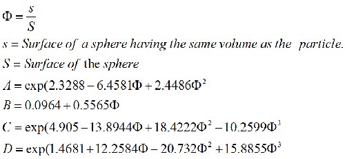
| Drag Coefficient for Spherical and Non-spherical Particles - Haider and Levenspiel |
| |
| Spheres |
 |
| |
| Non-spheres |
 |
 |
| |
| Multiple Particle Systems |
Solid 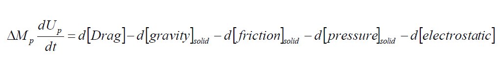 |
| |
Fluid 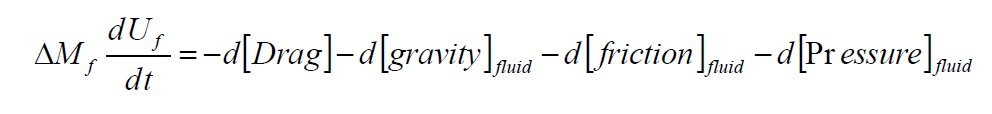 |
| |
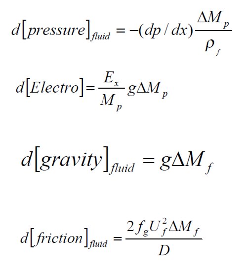
| The force balance can be further amplified and broken down in� individual equations for the solid and gas phases including frictional
forces, pressure and electrostatics. These equations can be summed
to obtain the final working equation.
|
| |
 |
| |
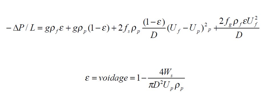
| When one combines the fluid and the particle balances, the final expression is the working expression for the overall pressure loss or energy loss for a pneumatic conveying system.
One should note term voidage in this equation. The voidage is the degree of filling the space with voids in a two phase gas-solid flow system. The closer the voidage is to 1.0 the closer to a single phase flow one experiences. Packed bed arrangements are low values for the voidage and the more the flow approaches dense phase conveying.
The expression given for the voidage depends on the solids flow rate and the particle velocity.
|
| |
| Definition: |
voidage ε - the fraction of bulk solid volume present as voids between particles.
Source: Jim Litster, Bryan Ennis, The Science and Engineering of Granulation Processes, Kluwer Academic Publishers, 2004.
|
|
| |
| Combining |
 |
| |
|
|
|
|
Resources:
At the top of each module is a set of buttons linking the user to reference material.
|


|
|
| Copyright © 2011, 2012 Ken Sochats |