Business Analysis

Introduction In this lesson we introduce some basic business analysis principles and concepts. Emergency management relies heavily on a business foundation in all phases: Planning, Preparedness, Response and Recovery. Some of the business areas that are directly relevant include: Economic decision making Finance Administration Resource Management Logistics Inventory and spare parts Legal and regulatory compliance

Emergency decision making, or indeed all real world decision making, exists in a constrained environment. We will never have the funding to address all potential emergencies. It is essential that we have some reasonable basis and methodology for allocating the funding that we do have among competing emergency needs.

Organizational Strategic Objectives

All organizations share at the higest level the same corporqate objectives. The table below summarizes and compares the main objectives for business and emergeency management.

Business      Emergency Management Survival      Survival Growth      Growth Share of Market      Share of Market Return on Investment (ROI)      Safety, Security

Business Functions

Accounting Recordkeeping Reporting Human Resources Recruiting Hiring Training Certification Promotion Removal Finance Investment Purchasing Leasing Grants Marketing Communications Sales Fundraising Taxes Subscription Operations

Operations Production      Time Frame      Criterion      Management      EM Phase Mass      Continuous      Efficiency      Quality Control (QC)      Preparation Batch      Interval                          Response Unit      One Time      Effectiveness      Quality Assurance (QC)      Recovery

Definition:     System life cycle: The cradle-to-grave journey of a system, comprising of broad phases such as conception, definition, design, testing, implementation, maintenance, modification or upgrading, and retirement or replacement. Source: www.businessdictionary.com/definition/system-life-cycle.html.

The figure below shows a typical life cycle curve for a system. The horizontal axis represents the age of the system and the vertical axis represents the level of activity that the system supports.

Systems Life Cycle

Our simplified version of the system life cycle has four phases: conception, growth, maturity and decay. The construction phase begins with the system design and ends with the system being fully implemented. For many large and complex systems, this phase can take several years and involve many people. After construction, the system enters a mature phase where the system is fully operational. This is the phase where the system should perform as designed. The duration of this phase depends on the design parameters employed, the excess capacity designed into the system and the rate of growth of load on the system. Sometimes the mature phase can be extended by making improvements in the network facilities and operating procedures or by adding new capacity or other facilities to the system. These are usually stopgap measures that have adverse effects on the integrity, efficiency and performance of the original design. The last phase, the decay phase, begins when the system's performance declines. This may be due to increased traffic load, the aging of system facilities causing increased downtime or requiring increased maintenance, suboptimal modifications to the system and other factors.

It is important for the emergency system designer to view the system from a life cycle perspective to appreciate how the system and its characteristics change over time and to appreciate those design parameters that can extend the life of the system.

Resources:     PC Magazine: www.pcmag.com/encyclopedia_term/0,2542,t=system+life+cycle&i=52404,00.asp Computerworld: www.computerworld.com/s/article/71151/System_Development_Life_Cycle

Breakeven Analysis

When going into a business or making a business decision, it is important to know whether the activity resulting from the decision will make a profit. In emergency management we are more likely to express our goals in terms of net benefits rather than profits.

Definition:     Break-Even Analysis: An analysis to determine the point at which revenue received equals the costs associated with receiving the revenue. Break-even analysis calculates what is known as a margin of safety, the amount that revenues exceed the break-even point. This is the amount that revenues can fall while still staying above the break-even point. Source: www.investopedia.com/terms/b/breakevenanalysis.asp#ixzz1nzZXfEQf.

Note that in the following discussions we are going to assume that the parameters such as costs, benefits, profits, are quantifiable and measurable. In emergency management, this is often problematic.

One technique for helping us predict whether an activity will be profitable or beneficial is breakeven analysis. Breakeven analysis attempts to find the point at which the costs incurred by entering into an activity and the revenues produced by the activity are equal (i.e., the breakeven point) during a given period. We will begin our discussion of breakeven analysis by using a simple linear model and later show how this model can be extended to nonlinear cases.

Costs

In breakeven analysis, we are concerned with two kinds of costs: fixed costs and variable costs. The total cost of any activity (TC) is the sum of its fixed (FC) and variable (VC) costs.

TC = FC + VC

Since we are assuming a linear model to begin with, the fixed costs are, of course, constant and the variable costs are a constant variable cost rate (VCR) times the usage (U).

VC = VCR * U

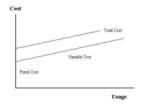
The graph below shows the relationship between the fixed, variable and total costs. Fixed costs are costs that are incurred even if no usage takes place. Rent, insurance, interest costs and certain taxes are examples of fixed costs. Variable costs are costs that result (and increase) from using the system. If the system is not used there are no variable costs utilities, labor costs, raw materials, supplies and some forms of maintenance are variable costs.

Cost Relationships

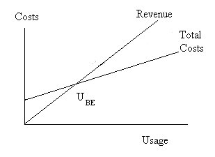
Cost Breakeven

In cases where the revenues are the same for two decision alternatives or the revenues are unknown or not easily estimated, it is possible to compare the decision alternatives on a cost basis alone. The breakeven point (UBE)occurs when the two total costs are equal. This is shown graphically below.

Cost Breakeven

Mathematically, the relation is expressed as:

TC1 = TC2

substituting the cost formulas:

FC1 + VCR1 * UBE = FC2 + VCR2 * UBE

solving for the breakeven activity

Example As an example, let us compare the cost structures of two options for servicing a fire station's extinguishers. The first service charges us a flat monthly rate of $1000.00 for recharging the bottles. Another service would charge us $23.00 for each bottle recharge plus a fixed charge for the bottles of $57.00.

To find the breakeven number of monthly recharges we use the formula:

Substituting in the values from our comparison:

UBE = (1000 - 57)/(23 - 0)

which results in:

UBE= 41

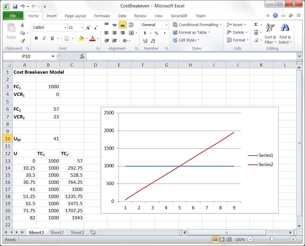
This means that if more than 41 extinguisher recharges are anticipated to be made in an average month, it is more economical to use the flat monthly service and if 41 or fewer recharges made on the average the less expensive alternative is to use the per recharge service.

The screenshot below shows a spreadsheet that can be used to calculate the cost breakeven. The spreadsheet has the daata from the example above already entered. Clicking on the image will open the spreadsheet in a new window.

Exercise:

Revenues (Benefits)

Revenues (R) arise from selling or charging for the fruits of the business activity. If we produce nothing, we have nothing to sell and receive no revenue. Since we are making a linear assumption, we produce and sell U units, we will receive U times the unit price (P) that we sell our product for.

R = U * P

The graph below shows the relationship between total revenues and quantity produced and sold.

Revenues

Profit

Profit p is defined as the excess revenues over cost. Mathematically, this would be:

p = TR - TC

As one can see, to increase profit two strategies are possible: increase revenue or decrease cost.

The Breakeven Point

At the point of breakeven the firm will break even (i.e. make no profit or loss). The total revenues will equal the total costs:

TR = TC

This is shown in The graph below.

The Breakeven Point

The figure above shows the breakeven point graphically. At sales levels above the breakeven level of sales, (UBE) Total revenues exceed total costs and the firm makes a profit. Below the breakeven sales point, the firm makes a loss since total costs are greater than the revenues produced. Thus, at the breakeven sales point (UBE), the firm makes no profit p .

p BE = 0

We can find the breakeven point graphically, as above, or calculate it algebraically from the formula above. Expanding this formula we get:

p BE = 0 = TR - TC = UBE*P - FC - UBE * VCR

Rearranging this and factoring (UBE) results in:

UBE = FC / {P - VCR}

Example

A small community wishes to install a burgular alarm monitoring system. The system will monitor businesses for fire, intrusion, provide a "panic" button and perform other sensing functions. The system has fixed costs of $81,000 per month and will require personnel and other costs of $300 per business per month. If businesses pay $800 per month, how many businesses must sign up to make the system break even?

The total cost of the alarm system will be:

TC = FC + VC = FC + VCR * U = 81,000 + 300 * U

and the total revenue from the alarm system will be:

R = P * U = $800 * U

and the profit at any number of subscribers will be:

p = R - TC = P * U - FC - VCR * U

p = (800- 300) * U - 81,000

p = 500 * U - 81,000

One can determine graphically that the breakeven point is 162 business subscribers, or algebraically by:

UBE = FC / (P - VCR)

UBE = 81,000 / ( 800 - 300)

UBE = 162

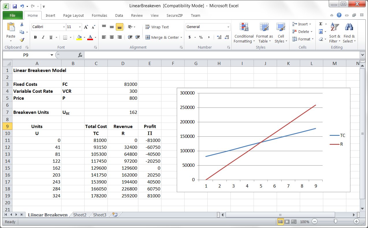
The screenshot below shows a spreadsheet that can be used to calculate the linear breakeven. The spreadsheet has the data from the example above already entered. Clicking on the image will open the spreadsheet in a new window.

Exercise:

Analysis of Breakeven Model Behavior

It is often useful for the designer/analyst to have an appreciation for how the model he or she is using behaves when the underlying model components change. We will start with the basic linear breakeven model reproduced below.

The Breakeven Model

Let us first assume that fixed costs change increasing by some amount D FC.

FC' = FC + D FC.

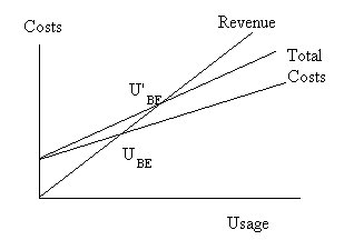
This is shown in the revised breakeven graph drawn below. As is shown in this graph, an increase (or decrease) in the fixed costs causes the total cost line to shift upward (or downward) parallel to the original total cost line. The required breakeven quantity (UBE) increases with an increase in fixed cost and decreases when fixed costs are reduced.

Increased Fixed Costs

A change in the variable cost rate is shown in the figure below. An increase (decrease) in the variable cost rate causes the total cost line to increase (decrease) in slope.

Increased Variable Costs

The point at which the total cost line intercepts the cost (vertical) axis remains the same. This point is equal to the amount of fixed costs. The required breakeven quantity (UBE) increases with increasing variable cost rates.

The revenue line is determined by the price (P) of the good or service. An increase or decrease in price causes the slope of the revenue line to increase or decrease. Increased revenue rates (slope) result in lower required breakeven quantities (UBE) and vice-versa. This is shown in the figure below.

Increased Revenue

Example

We can demonstrate the above analysis by expanding on our original alarm monitoring system analysis. The system has fixed costs of $81,000 per month and variable costs of $300 per business per month. The price of the system is $800 per month. At the breakeven point 162 businesses are needed to pay for the service.

Alarm System Breakeven Point

Suppose our variable costs increase such that our variable cost rate is $400 per month per business. Our breakeven level will increase to:

UBE = 81,000 / ( 800 - 400)

UBE = 203 businesses

This is shown in the chart below.

Alarm System Increased Cost

Suppose we wish to keep the breakeven level the same (i.e., 162) as before our cost increase. We can do this by increasing the price that we charge our customers. This is shown graphically below.

New Price for Same Breakeven

We can determine the new required price increase graphically from the chart above or by solving the breakeven formula for the new price.

P = FC / UBE + VCR

Thus, the new price must be:

P = FC / UBE + VCR

P = 81,000 / 162 + 400

P = 500 + 400

P = 900

Nonlinear Breakeven Models

In the real world things seldom behave in a linear fashion. There are many legitimate reasons why costs and revenues may not vary linearly. Quantity discounts will cause the costs of certain commodities to rise at a less than linear rate. Other costs, such as labor costs where overtime premiums may be paid, may increase at a rate faster than linear. The figure below shows linear and nonlinear cost curves.

Exercise:

Nonlinear Costs

Revenues can also vary nonlinearly. We may give discounts to our customers for increased levels of use.

Nonlinear Revenues

These can result in the breakeven situations shown in the following figure.

Nonlinear Breakeven

While the true relationships for costs and revenues may be complex and unknown, we can approximate with:

TC = FC + VCR * U + NVCR * U2

TR = P * U + NP * U2

where NVCR is a nonlinear variable cost coefficient and NP is a nonlinear price coefficient.

Profit is still defined as:

p = TR - TC

Substituting, we get:

p = (P - VCR) * U + (NP - NVCR) * U2 - FC

At breakeven, profit is zero, so we get:

0 = (P - VCR) * UBE + (NP - NVCR) * U2BE - FC

Since this formula is quadratic, we can possibly have two breakeven points. We will desalignate these as upper (UBEU) and lower (UBEL) breakeven points. We can solve the above formula by finding the roots to the equation using:

0 = ax2 + bx + c

r1,2 =

Substituting, we get:

UBEL =

UBEU =

Example

Suppose we have a nonlinear situation with $2755 fixed costs, $22 variable costs and a nonlinear cost coefficient of .00005. The price is $25 with a nonlinear price coefficient of -.0001. Total cost and revenues are:

TC = 2755 + 22 * U + .00005 * U

TR = 25 * U - .0001 * U2

Profit is:

p = 3 U - .00015 U2 - 2755

Using the quadratic root formulae, we get:

UBEL =

UBEU =

UBEU = 19035

UBEL = 964

Maximum Profit

Since the nonlinear case may produce a region of profitable production, we can calculate a maximum profit for those cases. We will desalignate the production point of maximum profit as Up MAX and the maximum profit as p MAX. This is shown in Figure 4.21.

Figure 4.21 Maximum Profit

We find the maximum of any function by taking its first derivative and setting it to zero.

This results in:

0 = (P - VCR) + 2 (NP - NVCR) * Up MAX

Solving for the point of maximum profit:

p MAX = {-(P - VCR)} / {2(NP - NVCR)}

For our example:

p MAX = {-(25 - 22)} / {2(-.0001 - .00005)}

Up MAX = 10,000

Maximum profit is then:

p MAX = (P - VCR) * Up MAX + (NP - NVCR) * Up MAX2 - FC

p MAX = (25 - 22) * 10,000 + (-.0001 - .00005) * 10,0002 - 2755

p MAX = $12,245

Exercise:

Present Value Analysis

Definition:     Present value: the value today of an amount of money in the future. Source: www.econlib.org/library/Enc/PresentValue.html.

Time is an important factor in many of the decisions we make. Consider the following options in acquiring a fire utility truck.

1. Purchase the truck for $47,000 and pay maintenance charges of $4,000 per year over its 10 year life.

2. Lease the truck for $9,000 per year (maintenance included) for 10 years.

3. Sign a lease/purchase agreement where we agree to pay $8,000 per year for the first 5 years in lease payments, purchase the truck in year 5 for $30,000 and pay $3,500 per year in maintenance in years 6 though 10.

In each of the cases above, the exchanges of money (cash flows) vary in amounts and timing. A naive analyst might simply add up the amounts and compose the total cash flows as shown below (assuming that the multiplexer has no salvage value at the end of it's life)

Option Total Cash Flow 1. Purchase $87,000 2. Lease $90,000 3. Lease/Purchase $87,500

Using this analysis, we would decide that purchasing the utility truck is the best option to pursue.

However, we are well aware that a dollar spent ten years from now is not "worth" as much as a dollar spent today. Looking at it from the opposite view, if we had a dollar today and invested it wisely, it would amount to several dollars in the future. What we must do with the analysis of our acquisition options is somehow convert the cash flows into equivalent dollars at some point in time. We could arbitrarily select a point in time and convert all of our cash flows into that time's dollars. Most frequently we use the present time as our standard, hence present value analysis. This makes sense because the decision among the options is made in the present time.

Let us now investigate how we can convert our future cash flow amounts into dollar values in the present. To do this, suppose that someone was willing to give us some dollar amount, CF, and that we could put this amount into an investment (the best we can find) that would grow at an interest rate, i. At the end of a year our dollar amount would grow to, or have a future value, FV, of:

FV = (1 + i) * CF

We should be indifferent then between receiving amount CF today and receiving amount FV one year from now. Or, in other words, (1 + i) * CF has the present value CF if it occurs in one year and the prevailing interest rate is, i. In present value analysis, we call this interest rate the discount rate because we use it to reduce or discount future cash flows. If CF had occurred at the end of a year, the amount that it would be worth today, its present value, PV would be:

PV = CF/(1 + i)

Applying the rules of compound interest, the future value of a current cash flow n years in the future is:

FV = (1 + i)n * CF

The present value of a cash flow in the 10th year would thus be:

PV = CF/(1 + i)10

We call the factor 1/(1 + i)n the present value factor (PVFi,n). The Present Value Table included in the supplemental tables lists the present value factors for a one dollar cash flow at various discount rates for up to 40 years. We can thus calculate the present value of any cash flow by:

PV = CF * PVFi,n

For example, if we are to receive a payment of $1,000 three years from now and the prevailing interest rate is 10%, then the present value of that $1,000 payment is:

PV = CF/(1 + i)n

PV = $1,000/(1 + .1)3

PV = $751.31

or, using the Present Value Table:

PV = CF * PVFi,n

PV = $1,000 * .7513

PV = $751.30

Note that we have to be careful to determine when the payments actually occur. If the payment occurs at the beginning of a period, a prepayment, we do not discount it for that particular period. If the payment occurs at the end of a period, we discount it for the period.

Very often cash flows occur in constant amounts for some number of regular intervals. We call such a cash flow stream an annuity. The present value of an annuity is simply the sum of the present values of the cash flows CF that comprise it.

PV = CF

As before we can express this equation as:

PV = CF * PVFAi,n

where PVFA is the present value factor for an annuity of n years at interest rate i, and is equal to:

PVFAi,n =

The Present Value Annuity Table gives the present value factors for one dollar annuities at various interest rates up to 40 years in duration.

We can now return to our original problem of evaluating the acquisition options for our multiplexer. We will assume in each of the options the prevailing interest rate is 12%. The first option, the Purchase option, consists of a simple cash flow in the present and a $2,000 10-year annuity. It's present value is thus:

PV = $17,000 + $2,000 * 5.6502

PV = $28,300.40

The Lease option is merely a ten year, $4,000 annuity.

PV = $4,000 * 5.6502

PV = $22,600.80

The final option, the Lease/Purchase alternative, can be analyzed as a ten year $1,500 annuity, a five year $3,500 annuity and a cash flow of $10,000 in the fifth year. This evaluates to:

PV = $1,500 * 5.6502 + $3,500 * 3.6048 + $10,000 * .5674

PV = $26,766.10

In this analysis, the Lease option evaluates to be the best of the three alternatives. The Purchase option, which was the best option under simple cash flow analysis, is the least economical when present values are considered.

The present values calculated in the above cases were all calculated on an annual basis. If payments are to be made monthly, we need to concern ourselves with how those payments are calculated. If the payments are merely monthly installments of an annual fee, i.e. one twelfth of the annual amount, the present values calculated on the annual amounts are correct. If, however, the payments are the result of a monthly period of interest calculation, then this must be taken into account. The formulas given above are merely used with a monthly period and a monthly interest rate.

Solar Energy Example

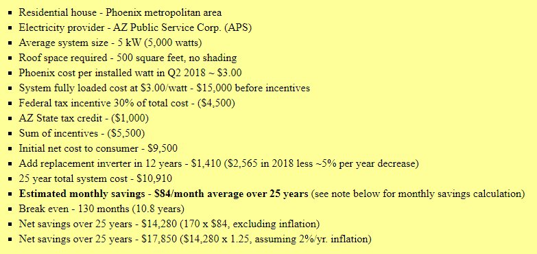
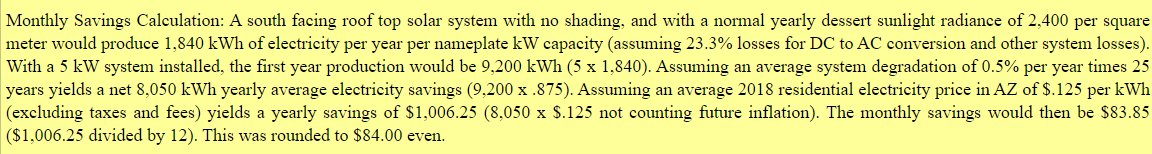
The following example was taken directly from a solar energy advocacy web site.

The Fine Print

It is important and instructive to examine this example in detail from multiple perspectives. This will enable us to apply some of the concepts and principles we learned in this course. First let's ask some modeling questions: Is basing the example in Phoenix representative of the rest of the US? How does the example of a residential house extend to multi-household apartment buildings? (Not to mention commercial facilities.) What percentage of houses have south facing roofs with 500 square feet of space? How would the example be different for rural areas. How many times is the word "assuming" used in the example. What other assumptions are made? (before, excluding, normal, average, estimated)

Life cycle questions: Is 25 years the Life Cycle for this system? Will the system have to be repaired or replaced at the end of its life? What is the residual value of the system after 25 years?

Ignored items: What maintenance must be regularly performed? (testing, cleaning, etc.) What damage might be done by storms and natural events? What about failures? What percentage of the time is the system operating at its full rating?

Time Value of Money (Present Value) Now let's factor in the fact that not all of our payments/savings occur at the same time or in the present. For comparative purposes, it is often informative to do a base calculation formed by considering what would happen if we did not make the solar system investment. This calculation and the following calculation are included in the spreadsheet SolarCostCalculations.xls. Essentially the base scenario is simply a 25 year annuity of payments for electrical service ($1,006.25) discounted at a rate of 5%. These are the exact numbers used in the example. The present value of this annuity of electrical costs is $14,542.53. The our economic solar investor should be indifferent between the 25 annual payments and $14,542.53. Next we map out the time sequence of cash flows for the Phoenix solar example given. The table following is the spreadsheet for the Phoenix example.

Year Investment Tax Credits Replacement Savings Net Present Value 1 $15,000.00 $1,100.00   $1,006.25 $12,893.75 $12,893.75 2   $1,100.00   $1,006.25 -$2,106.25 -$2,000.94 3   $1,100.00   $1,006.25 -$2,106.25 -$1,900.89 4   $1,100.00   $1,006.25 -$2,106.25 -$1,805.85 5   $1,100.00   $1,006.25 -$2,106.25 -$1,715.55 6     $1,006.25 -$1,006.25 -$778.62 7     $1,006.25 -$1,006.25 -$739.69 8     $1,006.25 -$1,006.25 -$702.70 9     $1,006.25 -$1,006.25 -$667.57 10     $1,006.25 -$1,006.25 -$634.19 11     $1,006.25 -$1,006.25 -$602.48 12     $2,565.00 $1,006.25 $1,558.75 $886.62 13     $1,006.25 -$1,006.25 -$543.74 14     $1,006.25 -$1,006.25 -$516.55 15     $1,006.25 -$1,006.25 -$490.72 16     $1,006.25 -$1,006.25 -$466.19 17     $1,006.25 -$1,006.25 -$442.88 18     $1,006.25 -$1,006.25 -$420.73 19     $1,006.25 -$1,006.25 -$399.70 20     $1,006.25 -$1,006.25 -$379.71 21     $1,006.25 -$1,006.25 -$360.73 22     $1,006.25 -$1,006.25 -$342.69 23     $1,006.25 -$1,006.25 -$325.56 24     $1,006.25 -$1,006.25 -$309.28 25     $1,006.25 -$1,006.25 -$293.81         -$3,060.38

Note that the $5,500 tax credits are amortized over 5 years. Neither the state or federal government will write you a check at the time of purchase. You are entitled to offset any taxes that you owe with this money. The time that it takes to do this is dependent on the individual situation of the taxpayer. For example Donald Trump who has an annual tax due of $750 would take 8 years to recover this credit. The bottom line is that the present value of the net cash flows is a savings of $3060.38. This does not take into account the cost issues mentioned earlier. The breakeven for this model is approximately 16.5 years.

Finally, let's take a look at the problem from a different perspective - the electric utility. From their point of view they lose annual revenue ($1,006.25) when a customer installs a solar system. In addition, they must provide energy to the customer when the customer's system is not generating electricity. In other words the electric utility serves as a backup for the customer. Thus the utility must build capacity to cover the needs of its customers. This capacity would be the same capacity that the utility would have to have if the customer produced no solar energy. We can compute a solar system reliability as the percent of time that the solar system is generating. Clearly, this reliability has to be less than 50%. The excess capacity that the utility must build is thus severly underutilized.

FORECASTING

Least Squares Linear Regression

One of the most popular techniques for forecasting future values from historical trend data is least squares linear regression. Least squares linear regression fits a straight line to a set of data such that the sum of the squares of the difference between the predicted and observed values is minimized. This line has the form:

Y = aX + b

where Y is the dependent variable (that which is to be predicted) and X is the independent variable. Thus, for any given X value we can predict a Y value given the parameters in the above formula.

The figure below shows a set of data points and a straight line fitted to those points.

Figure Least Squares Linear Regression

At each data point Yi there will be a difference between the data point value and the value predicted by the regression equation Yi. We refer to this difference term as an error term and calculate the error as:

ei = Yi - Yi

Our objective in fitting the straight line to the data is to produce a line that is as close to the data as possible. Therefore, we would like the error terms to be as small as possible. Note that simply adding the error terms together would produce a misleading result since some of the terms will be positive and some will be negative. We need a method of combining the error terms so that there effect is cumulative. The most common way of doing this is to use the square of the terms. We could use the absolute values of the terms, but the square has the added features of being analytic (we can take the derivative for minimization) and the square function penalizes large error differences. Thus, the formula for the sum of squares of the errors is:

We can substitute for the predicted dependent value Yi using the regression equation for a straight line.

Y = aX + b

The sum of squares of errors equation becomes:

In order to find the minimum of this function, we must take the derivative of the function and set the result to zero. Since this is a complex function, this is accomplished by taking the partial derivatives of the function with respect to the dependent variable Yi and the slope a.

Expanding each equation gives:

The partial derivatives result in two simultaneous equations:

These equations can be solved for the regression parameters a and b. The solutions are given below.

where:

Example

Suppose we have a set of data on the average monthly traffic on a link in a network during a year. The data contains an independent variable, the month M and a dependent variable, the average level of traffic T. We wish to use least squares linear regression to fit a straight line to the data so that we can forecast the next month's traffic on the network link. The regression equation will have the form:

T = aM + b

Table 4.1 gives the link traffic data.

Table 4.1 Network Link Average Monthly Traffic

Month (M) Traffic (T) 1 1050 2 1120 3 980 4 1110 5 1200 6 900 7 1040 8 990 9 1200 10 1190 11 1170 12 1080

From this we get:

a = 7.727

and

b = 1035.60

The regression equation becomes:

T = 7.727M + 1035.60

The predicted traffic in the next or 13th month would be:

T = 7.727(13) + 1035.60

T = 1136.05

Regression Solution Calculations

Month (M) Traffic (T) M2 MT 1 1050 1 1050 2 1120 4 2240 3 980 9 2940 4 1110 16 4440 5 1200 25 6000 6 900 36 5400 7 1040 49 7280 8 990 64 7920 9 1200 81 10800 10 1190 100 11900 11 1170 121 12870 12 1080 144 12960

S Mi = 78, S Ti = 13030, S Mi2 = 650, S MiTi = 85800

M'= 6.5, T' = 1085.833, ,

Averages

Another family of techniques for forecasting values for network variables is averages. In this section, we will examine three averages techniques: simple moving averages, weighted moving averages and exponential smoothing. As we will see, averages are useful in that they not only give us the forecasted value for a variable but also give a smoothed representation of the original data.

Simple Moving Averages (SMA)

In the simple moving average technique (SMA), the forecasted value for a variable in a period is the arithmetic mean of the values for that variable for some number of prior periods. The simple moving average forecast for a variable x in period j is given by:

Xj =

where Xj is the forecasted value, n is the number of periods in the average and xj - i is the observed value in period (j - i). Table 4.3 below shows the simple moving averages for the network traffic example originally given in Table 4.1 using a three period simple moving average.

Network Link Simple Moving Average Monthly Traffic

Month (M) Traffic (T) SMA 1 1050   2 1120   3 980   4 1110 1050 5 1200 1070 6 900 1097 7 1040 1070 8 990 1047 9 1200 977 10

Simple Moving Averages

The degree of smoothing is a function of the number of periods included in the average. If fewer periods are included, the simple moving averages have less and less variability than the original data and lag the original data more and more in time.

Weighted Moving Averages (WMA)

Weighted moving averages (WMA) are a superset of simple moving averages. The forecasted value for a variable in a period is the weighted arithmetic mean of the values for that variable for some number of prior periods. The weighted moving average forecast for a variable x in period j is given by:

Xj =

where Xj is the forecasted value, n is the number of periods in the average, xj - i is the observed value in period (j - i) and wi is the weight applied to that observation. These weights must sum to one.

Simple moving averages is simply a special instance of weighted moving averages where all of the weights are equal.

Table 4.4 below shows the weighted moving averages for the network traffic example originally given in Table 4.1 using a four period weighted moving average with weights of (.4, .3, .2, .1) from most recent period.

Figure 4.26 shows the relationship between the original observations and the forecasted values. As in the simple moving average, the forecasted values, because they result from multiple observations, have less variability than the original observations. The degree of smoothing is again a function of the number of periods included in the average. If fewer periods are included, the simple moving averages have less and less variability than the original data and lag the original data more and more in time. The degree of lag and smoothing is also a function of the distribution of weights. Forecasters often adjust the weights and number of periods used in the averages to get the desired forecasting and smoothing effects.

Network Link Weighted Moving Average Monthly Traffic

Month (M) Traffic (T) WMA 1 1050   2 1120   3 980   4 1110   5 1200 1067 6 900 1121 7 1040 1040 8 990 1037 9 1200 1008 10 1190 1075 11 1170 1138 12 1080 1164 13   1141

Figure 4.26 Weighted Moving Averages

Exponential Smoothing

In exponential smoothing the forecasted value for a variable in a period is the weighted arithmetic mean of the values for that variable in the immediately preceding period and the variable's forecast for the preceding period. The exponential smoothing forecast for a variable x in period j is given by:

where Xj is the forecasted value in period j, xj - 1 is the observed value in period (j - 1) and Xj - 1 is the forecasted value in period (j - 1). a is a weight that must have a value between one and zero.

The technique is called exponential smoothing because the forecast for any period is the weighted sum of the observed value for the previous period plus the values of the variable for the previous periods times the weight, a , to the power of the number of periods in the past. This can be shown by taking the above formula and expanding the estimated value for the previous period Xj-1.

Substituting this into the first equation we get:

In a similar manner, the term Xj-2 can be expanded and so on. The result is that any forecasted value is the weighted sum of previous observations and the original estimated value. Note that the sum of the weights is still one.

Table 4.5 below shows the exponential smoothing forecasts for the network traffic example originally given in Table 4.1 using weight of .6 and an initial forecast of 1000.

Network Link Exponentially Smoothed Monthly Traffic

Month (M) Traffic (T) ES 1 1050 1000 2 1120 1030 3 980 1084 4 1110 1022 5 1200 1075 6 900 1150 7 1040 1000 8 990 1024 9 1200 1004 10 1190 1122 11 1170 1163 12 1080 1167 13 1115

Figure 4.27 shows the relationship between the original observations and the forecasted values. As in the previous techniques, the forecasted values, because they result from multiple observations, have less variability than the original observations. The degree of smoothing is predominantly a function of the weight. It is also a function of the initial forecast. However, after a few periods of forecasts, the weight of this term becomes insalignificant.

Exponential Smoothing

Definition:     : Source: .

Exercise:

Resources:     Etna web site: http://www.etnaborough.org/ National Flood Insurance Program: http://www.floodsmart.gov.

Copyright © 2011 - 2014 Ken Sochats