 |
| Simulation |
|
  

|

|
|
|
| |
|
Introduction
In the previous lesson we developed a mathematical model of a single processor queue system. This model provided us with much useful information about the performance of such systems. However, the applicability of this model was limited by the assumptions necessary to simplify the model.
In this chapter we will construct a model of the same single processor queue system using the technique of simulation. This model will avoid the assumptions made in the previous model and, thus, will have wider applicability. Later in the chapter we will expand the single processor model to encompass different queue disciplines, limited queue sizes and other system design options. We will also show to modify the model to handle series and parallel multiprocessor queuing systems.
Queuing Theory Assumptions
- Infinite Arrival Population
- Markov Arrivals
- Infinite Queue Size
- FIFO Queue Discipline
- Infinite Run Time
- Utilization < 1.0
|
| |
| Definition: |
Simulation: In its narrowest sense, a computer simulation is a program that is run on a computer and that uses step-by-step methods to explore the approximate behavior of a mathematical model. Usually this is a model of a real-world system (although the system in question might be an imaginary or hypothetical one).
Source:
Stanford Encyclopedia of Philosophy https://plato.stanford.edu/entries/simulations-science. |
|
| |
| Single Processor Model |
| |
The figure below shows the same single processor queue system model that we studied in the last chapter. The model consists of a processor at which transactions arrive for processing. If an arriving transaction finds the processor busy, the transaction must wait in a queue, otherwise the transaction is processed immediately. After processing a transaction departs the system. If there are other transactions waiting in the queue, one of them is selected for processing using some rule or queue discipline, otherwise the system becomes idle.
In order to build an explicit model of the behavior of this system, we need to examine how the system changes and acts over time. Clearly, the system does nothing until an arrival occurs, so let us begin by following an arriving transaction (character, packet, etc.) through the system. At each step along the way we will note what is happening within the system.
|
| |
| Single Processor Queue Model |
 |
| |
| Arrivals |
| |
| Arrivals occur as a process. When an arrival occurs, we know that another arrival will occur some time in the future. In our simulation model, we will assume that we can predict, based on some random distribution, when the next arrival will occur. In last chapter's model we assumed that the distribution of arrivals was governed by the Poisson distribution. We need not adhere to that assumption in the simulation model. We can elect to use any random distribution to control the arrival process, or, we can use arrival data taken from an actual system. Later, we will demonstrate how arrivals can be generated from a uniform distribution and then from any random distribution.
The flowchart below shows what happens in the system when an arrival occurs. At the time of the arrival, we can predict when the next arrival will occur. We will record this prediction in a future events table that we will call a schedule. The arriving transaction will either be processed or wait in the queue. This depends on the preexisting status of the processor. If the processor is idle, the transaction proceeds directly into the processor and begins its service. It will depart at some later time that we assume we can predict from some random distribution. These departure predictions will be entered onto the schedule of future events. If the processor is busy, the transaction enters the queue to wait for processing at a later time. For the time being, we will use a simple queue discipline that merely counts the number in the queue. Later we will demonstrate how very sophisticated queue disciplines can be simulated. This represents everything that happens at the time that an arrival occurs. |
| |
| Arrivals |
 |
| |
| Departures |
| |
| The other event that causes action in the single processor system is a departure. The flowchart below shows the process that takes place upon a departure.
Upon a departure, the transaction being serviced leaves the processor. If no other transaction is waiting in the queue, the system becomes idle. If there is one or more transactions in the queue, then the next transaction to be processed is removed from the queue and its processing begins. The removal from the queue is done in accordance with the queue discipline. In our simple model we will not differentiate items selected from the queue. This will be addressed later in the chapter. Once again, we can predict when that transaction will depart the system and place that future event on the schedule table. |
| |
| Departures |
 |
| |
| Our simulation thus tracks what happens to each transaction as it proceeds through the system. To do this we need two data recording structures. The first handles the schedule. It records the future events and the times at which they occur. The schedule is shown in the table below. |
| |
|
| |
| The second data structure records the state of the system as events occur. We will call this the History Table and it is shown in the table below. Recorded in the History Table are the event, the time that the event occurred, the status of the processor and the number of transactions in the queue. We will use this data to calculate the same system performance parameters that we calculated in the last chapter. |
| |
| The History Table |
| Time | Event | Processor
Status | Queue
Length |
| | | | |
|
| Control |
| |
| What we need now is a main control procedure. A typical control procedure is given in the flowchart below. This control algorithm is not too different from the actual operating system for a large number of types of communications processors. The first step in the algorithm is the initialization of variables. |
| |
This includes:
- The type and parameters of the arrival and departure random distributions.
- The starting conditions. This includes the starting time, the current event (usually a start (S) event), the processor status and the queue length. In actuality, any starting conditions could be specified. However, as a default we will use as starting conditions the case where the time clock starts at time 0.0, there is no current event in processing, the processor is idle and the queue is empty. The History Table for these default initial conditions is shown in the table below.
- The ending time. An special event called the end event is inserted into the schedule at a time corresponding to the desired duration of the simulation. The end event does nothing but cause the simulation to terminate. A Schedule with a sample end event is also shown in the table below.
|
| Initial Conditions |
| |
| History Table |
| Time | Event | Processor
Status | Queue
Length |
| 0.00 | S | Idle | 0 |
| | Schedule |
| Time | Event |
| 0.00 | S |
| 50.0 | E |
|
|
| |
| The Main Control Algorithm |
 |
| In order for anything to happen in the system an arrival must occur. Thus, we prime the simulation by generating an initial arrival and enter it onto the schedule. The next portion of the algorithm consists of a loop that ticks the system clock to the time of the next event in time on the Schedule. If the event is an arrival or departure (not the end event), we perform the activities associated with the event as depicted in their algorithms. Upon completion of the respective arrival or departure routine, we return to the main algorithm and advance time once again to the event with the next closest time. If that event is the end event then we terminate the simulation and calculate the required performance statistics. |
| |
| A Sample Simulation |
| |
| Let us consider an example problem to demonstrate the simulation process. Suppose we have a simple single processor system with transactions arriving at its input every 3 to 5 milliseconds uniformly distributed. The processor can process these in 4 to 6 milliseconds (uniform). These distributions are shown in the figure below. We wish to simulate this system for 50 milliseconds of operation and we will use the default initial conditions shown in the table above. |
| |
| Arrival and Service Distributions |
 |
| As shown in the main algorithm below, after recording the initial conditions we must schedule the first arrival. In other words, we need to generate a random number from the arrival distribution (3 to 5 milliseconds between arrivals with a uniform distribution) that represents the time of the first arrival. There are several methods available for generating random numbers. Many programming languages have routines or facilities for producing random numbers. A problem exists, however, in that there are an infinite number of types and parameters of distributions from which random selections can be taken. |
| Most computer programs and languages have a built-in uniform random number generator that generates random numbers from the standard uniform distribution. The standard uniform distribution has a range from zero to one. Appendix A.4 contains random numbers generated by a typical computer uniform random number generator. Random Number Table |
| |
| The Standard Uniform Random Distribution |
 |
| |
| |
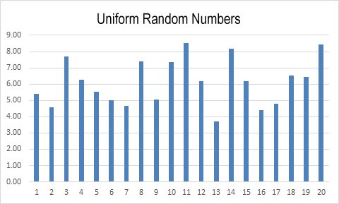
| Microsoft Excel has a built-in random number function (RAND) that generates random numbers ranging from 0 to 1. The spreadsheet
Excel Random Number Generator incorporates a random number sample spreadsheet. The image below shows the results of a run of this program.
|
| |
 |
| |
| Non Uniform Random Numbers |
| |
| We can also apply the Central limit Theorem to obtain samples that are Normally distributed. Conversion techniques are also available to convert our Uniform random numbers into any distribution desired. |
| |
| Definition: |
Central Limit Theorem: The central limit theorem states that if you have a population with mean μ and standard deviation σ and take sufficiently large random samples from the population with replacement, then the distribution of the sample means will be approximately normally distributed. This will hold true regardless of whether the source population is normal or skewed, provided the sample size is sufficiently large (usually n > 30). If the population is normal, then the theorem holds true even for samples smaller than 30.
Source: Boston University School of Public Health https://sphweb.bumc.bu.edu/
|
|
| |
 |
| |
| There are other similar techniques that will allow us to convert our uniform numbers to random selections from exponential or other random distributions. |
| |
| Non Standard Uniform Random Numbers |
| |
| Our problem now is to convert selections from this standard uniform distribution to the particular uniform distributions that we are going to use in our simulation. This is done using the formula: |
| |
| |
| X = Xlow + (Xhigh - Xlow) * U |
| |
| where Xlow is the lower bound of the uniform range, Xhigh is the upper bound of the uniform range and U is a random selection from the standard uniform distribution. |
| For example, a random selection for our example problem arrival distribution is calculated using: |
| |
| A = 3 + 2 * U |
| |
| A standard uniform random pick of zero would translate into a pick of three on our arrival distribution; a standard uniform random pick of one would translate into an arrival time of five; a standard uniform random pick of one half would translate into an arrival time of four, etc. Departure times would be calculated in a similar manner using the formula: |
| |
| D = 4 + 2 * U |
| |
| The example problem simulation shown in Table 13.4 was generated using the random number table given in Appendix A.4. Each random number was obtained by taking two digits from the table at a time starting at the first position and proceeding from left to right and top to bottom. |
| Thus, the first arrival is calculated by taking the first uniform random number (.60) and inserting it into the arrival distribution formula: |
| |
| A = 3 + 2 * (.60) = 4.20 |
| |
| This is shown as the first step of the simulation in the table below. This table gives the simulation history in a step-by-step fashion. |
| |
| Example Simulation |
| |
Parameters
- Start Time 0.0
- End Time 50.0
- Processor Status Idle
- Queue Length 0
- Arrival Distribution - Uniform (2 - 5)
- Departure Distribution - Uniform (4 - 6)
|
| |
| FIRST ARRVAL SCHEDULED |
| |
| History Table |
| Time | Event | Processor
Status | Queue
Length |
| 0.00 | S | Idle | 0 |
| | Schedule |
| Time | Event |
| 0.00 | S |
| 50.0 | E |
| 4.20 | A |
|
|
| |
| PROCESS FIRST ARRIVAL |
- Schedule next arrival
- Schedule first arrival's departure
|
| History Table |
| Time | Event | Processor
Status | Queue
Length |
| 0.00 | S | Idle | 0 |
| 4.20 | A | Busy | 0 |
| | Schedule |
| Time | Event |
| 0.00 | S |
| 50.0 | E |
| 4.20 | A |
| 7.90 | A |
| 8.92 | D |
|
|
| |
| PROCESS NEXT EVENT - ARRIVAL |
- Schedule next arrival
- Increment queue
|
| History Table |
| Time | Event | Processor
Status | Queue
Length |
| 0.00 | S | Idle | 0 |
| 4.20 | A | Busy | 0 |
| 7.90 | A | Busy | 1 |
| | Schedule |
| Time | Event |
| 0.00 | S |
| 50.0 | E |
| 4.20 | A |
| 7.90 | A |
| 8.92 | D |
| 13.36 | A |
|
|
| |
| PROCESS NEXT EVENT - DEPARTURE |
- Extract one from queue
- Schedule a departure
|
| History Table |
| Time | Event | Processor
Status | Queue
Length |
| 0.00 | S | Idle | 0 |
| 4.20 | A | Busy | 0 |
| 7.90 | A | Busy | 1 |
| 8.92 | D | Busy | 0 |
| | Schedule |
| Time | Event |
| 0.00 | S |
| 50.0 | E |
| 4.20 | A |
| 7.90 | A |
| 8.92 | D |
| 13.36 | A |
| 14.60 | D |
|
|
| |
| PROCESS NEXT EVENT - ARRIVAL |
- Schedule next arrival
- Increment queue
|
| History Table |
| Time | Event | Processor
Status | Queue
Length |
| 0.00 | S | Idle | 0 |
| 4.20 | A | Busy | 0 |
| 7.90 | A | Busy | 1 |
| 8.92 | D | Busy | 0 |
| 13.36 | A | Busy | 1 |
| | Schedule |
| Time | Event |
| 0.00 | S |
| 50.0 | E |
| 4.20 | A |
| 7.90 | A |
| 8.92 | D |
| 13.36 | A |
| 14.60 | D |
| 17.88 | A |
|
|
| |
| PROCESS NEXT EVENT - DEPARTURE |
- Extract one from queue
- Schedule a departure
|
| History Table |
| Time | Event | Processor
Status | Queue
Length |
| 0.00 | S | Idle | 0 |
| 4.20 | A | Busy | 0 |
| 7.90 | A | Busy | 1 |
| 8.92 | D | Busy | 0 |
| 13.36 | A | Busy | 1 |
| 14.60 | D | Busy | 0 |
| | Schedule |
| Time | Event |
| 0.00 | S |
| 50.0 | E |
| 4.20 | A |
| 7.90 | A |
| 8.92 | D |
| 13.36 | A |
| 14.60 | D |
| 17.88 | A |
| 19.54 | D |
|
|
| |
| PROCESS NEXT EVENT - ARRIVAL |
- Schedule next arrival
- Increment queue
|
| History Table |
| Time | Event | Processor
Status | Queue
Length |
| 0.00 | S | Idle | 0 |
| 4.20 | A | Busy | 0 |
| 7.90 | A | Busy | 1 |
| 8.92 | D | Busy | 0 |
| 13.36 | A | Busy | 1 |
| 14.60 | D | Busy | 0 |
| 17.88 | A | Busy | 1 |
| | Schedule |
| Time | Event |
| 0.00 | S |
| 50.0 | E |
| 4.20 | A |
| 7.90 | A |
| 8.92 | D |
| 13.36 | A |
| 14.60 | D |
| 17.88 | A |
| 19.54 | D |
| 22.60 | A |
|
|
| |
| PROCESS NEXT EVENT - DEPARTURE |
- Extract one from queue
- Schedule a departure
|
| History Table |
| Time | Event | Processor
Status | Queue
Length |
| 0.00 | S | Idle | 0 |
| 4.20 | A | Busy | 0 |
| 7.90 | A | Busy | 1 |
| 8.92 | D | Busy | 0 |
| 13.36 | A | Busy | 1 |
| 14.60 | D | Busy | 0 |
| 17.88 | A | Busy | 1 |
| 19.54 | D | Busy | 0 |
| | Schedule |
| Time | Event |
| 0.00 | S |
| 50.0 | E |
| 4.20 | A |
| 7.90 | A |
| 8.92 | D |
| 13.36 | A |
| 14.60 | D |
| 17.88 | A |
| 19.54 | D |
| 22.60 | A |
| 24.02 | D |
|
|
| |
| PROCESS NEXT EVENT - ARRIVAL |
- Schedule next arrival
- Increment queue
|
| History Table |
| Time | Event | Processor
Status | Queue
Length |
| 0.00 | S | Idle | 0 |
| 4.20 | A | Busy | 0 |
| 7.90 | A | Busy | 1 |
| 8.92 | D | Busy | 0 |
| 13.36 | A | Busy | 1 |
| 14.60 | D | Busy | 0 |
| 17.88 | A | Busy | 1 |
| 19.54 | D | Busy | 0 |
| 22.60 | A | Busy | 1 |
| | Schedule |
| Time | Event |
| 0.00 | S |
| 50.0 | E |
| 4.20 | A |
| 7.90 | A |
| 8.92 | D |
| 13.36 | A |
| 14.60 | D |
| 17.88 | A |
| 19.54 | D |
| 22.60 | A |
| 24.02 | D |
| 25.90 | A |
|
|
| |
| PROCESS NEXT EVENT - DEPARTURE |
- Extract one from queue
- Schedule a departure
|
| History Table |
| Time | Event | Processor
Status | Queue
Length |
| 0.00 | S | Idle | 0 |
| 4.20 | A | Busy | 0 |
| 7.90 | A | Busy | 1 |
| 8.92 | D | Busy | 0 |
| 13.36 | A | Busy | 1 |
| 14.60 | D | Busy | 0 |
| 17.88 | A | Busy | 1 |
| 19.54 | D | Busy | 0 |
| 22.60 | A | Busy | 1 |
| 24.02 | D | Busy | 0 |
| | Schedule |
| Time | Event |
| 0.00 | S |
| 50.0 | E |
| 4.20 | A |
| 7.90 | A |
| 8.92 | D |
| 13.36 | A |
| 14.60 | D |
| 17.88 | A |
| 19.54 | D |
| 22.60 | A |
| 24.02 | D |
| 25.90 | A |
| 28.56 | D |
|
|
| |
| PROCESS NEXT EVENT - ARRIVAL |
- Schedule next arrival
- Increment queue
|
| History Table |
| Time | Event | Processor
Status | Queue
Length |
| 0.00 | S | Idle | 0 |
| 4.20 | A | Busy | 0 |
| 7.90 | A | Busy | 1 |
| 8.92 | D | Busy | 0 |
| 13.36 | A | Busy | 1 |
| 14.60 | D | Busy | 0 |
| 17.88 | A | Busy | 1 |
| 19.54 | D | Busy | 0 |
| 22.60 | A | Busy | 1 |
| 24.02 | D | Busy | 0 |
| 25.90 | A | Busy | 1 |
| | Schedule |
| Time | Event |
| 0.00 | S |
| 50.0 | E |
| 4.20 | A |
| 7.90 | A |
| 8.92 | D |
| 13.36 | A |
| 14.60 | D |
| 17.88 | A |
| 19.54 | D |
| 22.60 | A |
| 24.02 | D |
| 25.90 | A |
| 28.56 | D |
| 30.04 | A |
|
|
| |
| PROCESS NEXT EVENT - DEPARTURE |
- Extract one from queue
- Schedule a departure
|
| History Table |
| Time | Event | Processor
Status | Queue
Length |
| 0.00 | S | Idle | 0 |
| 4.20 | A | Busy | 0 |
| 7.90 | A | Busy | 1 |
| 8.92 | D | Busy | 0 |
| 13.36 | A | Busy | 1 |
| 14.60 | D | Busy | 0 |
| 17.88 | A | Busy | 1 |
| 19.54 | D | Busy | 0 |
| 22.60 | A | Busy | 1 |
| 24.02 | D | Busy | 0 |
| 25.90 | A | Busy | 1 |
| 28.36 | D | Busy | 0 |
| | Schedule |
| Time | Event |
| 0.00 | S |
| 50.0 | E |
| 4.20 | A |
| 7.90 | A |
| 8.92 | D |
| 13.36 | A |
| 14.60 | D |
| 17.88 | A |
| 19.54 | D |
| 22.60 | A |
| 24.02 | D |
| 25.90 | A |
| 28.56 | D |
| 30.04 | A |
| 32.74 | D |
|
|
| |
| PROCESS NEXT EVENT - ARRIVAL |
- Schedule next arrival
- Increment queue
|
| History Table |
| Time | Event | Processor
Status | Queue
Length |
| 0.00 | S | Idle | 0 |
| 4.20 | A | Busy | 0 |
| 7.90 | A | Busy | 1 |
| 8.92 | D | Busy | 0 |
| 13.36 | A | Busy | 1 |
| 14.60 | D | Busy | 0 |
| 17.88 | A | Busy | 1 |
| 19.54 | D | Busy | 0 |
| 22.60 | A | Busy | 1 |
| 24.02 | D | Busy | 0 |
| 25.90 | A | Busy | 1 |
| 28.36 | D | Busy | 0 |
| 30.04 | A | Busy | 1 |
| | Schedule |
| Time | Event |
| 0.00 | S |
| 50.0 | E |
| 4.20 | A |
| 7.90 | A |
| 8.92 | D |
| 13.36 | A |
| 14.60 | D |
| 17.88 | A |
| 19.54 | D |
| 22.60 | A |
| 24.02 | D |
| 25.90 | A |
| 28.56 | D |
| 30.04 | A |
| 32.74 | D |
| 34.96 | A |
|
|
| |
| PROCESS NEXT EVENT - DEPARTURE |
- Extract one from queue
- Schedule a departure
|
| History Table |
| Time | Event | Processor
Status | Queue
Length |
| 0.00 | S | Idle | 0 |
| 4.20 | A | Busy | 0 |
| 7.90 | A | Busy | 1 |
| 8.92 | D | Busy | 0 |
| 13.36 | A | Busy | 1 |
| 14.60 | D | Busy | 0 |
| 17.88 | A | Busy | 1 |
| 19.54 | D | Busy | 0 |
| 22.60 | A | Busy | 1 |
| 24.02 | D | Busy | 0 |
| 25.90 | A | Busy | 1 |
| 28.36 | D | Busy | 0 |
| 30.04 | A | Busy | 1 |
| 32.74 | D | Busy | 0 |
| | Schedule |
| Time | Event |
| 0.00 | S |
| 50.0 | E |
| 4.20 | A |
| 7.90 | A |
| 8.92 | D |
| 13.36 | A |
| 14.60 | D |
| 17.88 | A |
| 19.54 | D |
| 22.60 | A |
| 24.02 | D |
| 25.90 | A |
| 28.56 | D |
| 30.04 | A |
| 32.74 | D |
| 34.96 | A |
| 38.68 | D |
|
|
| |
| PROCESS NEXT EVENT - ARRIVAL |
- Schedule next arrival
- Increment queue
|
| History Table |
| Time | Event | Processor
Status | Queue
Length |
| 0.00 | S | Idle | 0 |
| 4.20 | A | Busy | 0 |
| 7.90 | A | Busy | 1 |
| 8.92 | D | Busy | 0 |
| 13.36 | A | Busy | 1 |
| 14.60 | D | Busy | 0 |
| 17.88 | A | Busy | 1 |
| 19.54 | D | Busy | 0 |
| 22.60 | A | Busy | 1 |
| 24.02 | D | Busy | 0 |
| 25.90 | A | Busy | 1 |
| 28.36 | D | Busy | 0 |
| 30.04 | A | Busy | 1 |
| 32.74 | D | Busy | 0 |
| 34.96 | A | Busy | 1 |
| | Schedule |
| Time | Event |
| 0.00 | S |
| 50.0 | E |
| 4.20 | A |
| 7.90 | A |
| 8.92 | D |
| 13.36 | A |
| 14.60 | D |
| 17.88 | A |
| 19.54 | D |
| 22.60 | A |
| 24.02 | D |
| 25.90 | A |
| 28.56 | D |
| 30.04 | A |
| 32.74 | D |
| 34.96 | A |
| 38.68 | D |
| 38.44 | A |
|
|
| |
| PROCESS NEXT EVENT - ARRIVAL |
- Schedule next arrival
- Increment queue
|
| History Table |
| Time | Event | Processor
Status | Queue
Length |
| 0.00 | S | Idle | 0 |
| 4.20 | A | Busy | 0 |
| 7.90 | A | Busy | 1 |
| 8.92 | D | Busy | 0 |
| 13.36 | A | Busy | 1 |
| 14.60 | D | Busy | 0 |
| 17.88 | A | Busy | 1 |
| 19.54 | D | Busy | 0 |
| 22.60 | A | Busy | 1 |
| 24.02 | D | Busy | 0 |
| 25.90 | A | Busy | 1 |
| 28.36 | D | Busy | 0 |
| 30.04 | A | Busy | 1 |
| 32.74 | D | Busy | 0 |
| 34.96 | A | Busy | 1 |
| 38.44 | A | Busy | 2 |
| | Schedule |
| Time | Event |
| 0.00 | S |
| 50.0 | E |
| 4.20 | A |
| 7.90 | A |
| 8.92 | D |
| 13.36 | A |
| 14.60 | D |
| 17.88 | A |
| 19.54 | D |
| 22.60 | A |
| 24.02 | D |
| 25.90 | A |
| 28.56 | D |
| 30.04 | A |
| 32.74 | D |
| 34.96 | A |
| 38.68 | D |
| 38.44 | A |
| 41.46 | A |
|
|
| |
| PROCESS NEXT EVENT - DEPARTURE |
- Extract one from queue
- Schedule a departure
|
| History Table |
| Time | Event | Processor
Status | Queue
Length |
| 0.00 | S | Idle | 0 |
| 4.20 | A | Busy | 0 |
| 7.90 | A | Busy | 1 |
| 8.92 | D | Busy | 0 |
| 13.36 | A | Busy | 1 |
| 14.60 | D | Busy | 0 |
| 17.88 | A | Busy | 1 |
| 19.54 | D | Busy | 0 |
| 22.60 | A | Busy | 1 |
| 24.02 | D | Busy | 0 |
| 25.90 | A | Busy | 1 |
| 28.36 | D | Busy | 0 |
| 30.04 | A | Busy | 1 |
| 32.74 | D | Busy | 0 |
| 34.96 | A | Busy | 1 |
| 38.44 | A | Busy | 2 |
| 38.68 | D | Busy | 1 |
| | Schedule |
| Time | Event |
| 0.00 | S |
| 50.0 | E |
| 4.20 | A |
| 7.90 | A |
| 8.92 | D |
| 13.36 | A |
| 14.60 | D |
| 17.88 | A |
| 19.54 | D |
| 22.60 | A |
| 24.02 | D |
| 25.90 | A |
| 28.56 | D |
| 30.04 | A |
| 32.74 | D |
| 34.96 | A |
| 38.68 | D |
| 38.44 | A |
| 41.46 | A |
| 43.96 | A |
|
|
| |
| PROCESS NEXT EVENT - ARRIVAL |
- Schedule next arrival
- Increment queue
|
| History Table |
| Time | Event | Processor
Status | Queue
Length |
| 0.00 | S | Idle | 0 |
| 4.20 | A | Busy | 0 |
| 7.90 | A | Busy | 1 |
| 8.92 | D | Busy | 0 |
| 13.36 | A | Busy | 1 |
| 14.60 | D | Busy | 0 |
| 17.88 | A | Busy | 1 |
| 19.54 | D | Busy | 0 |
| 22.60 | A | Busy | 1 |
| 24.02 | D | Busy | 0 |
| 25.90 | A | Busy | 1 |
| 28.36 | D | Busy | 0 |
| 30.04 | A | Busy | 1 |
| 32.74 | D | Busy | 0 |
| 34.96 | A | Busy | 1 |
| 38.44 | A | Busy | 2 |
| 38.68 | D | Busy | 1 |
| 41.46 | A | Busy | 2 |
| | Schedule |
| Time | Event |
| 0.00 | S |
| 50.0 | E |
| 4.20 | A |
| 7.90 | A |
| 8.92 | D |
| 13.36 | A |
| 14.60 | D |
| 17.88 | A |
| 19.54 | D |
| 22.60 | A |
| 24.02 | D |
| 25.90 | A |
| 28.56 | D |
| 30.04 | A |
| 32.74 | D |
| 34.96 | A |
| 38.68 | D |
| 38.44 | A |
| 41.46 | A |
| 43.96 | D |
| 46.18 | A |
|
|
| |
| PROCESS NEXT EVENT - DEPARTURE |
- Extract one from queue
- Schedule a departure
|
| History Table |
| Time | Event | Processor
Status | Queue
Length |
| 0.00 | S | Idle | 0 |
| 4.20 | A | Busy | 0 |
| 7.90 | A | Busy | 1 |
| 8.92 | D | Busy | 0 |
| 13.36 | A | Busy | 1 |
| 14.60 | D | Busy | 0 |
| 17.88 | A | Busy | 1 |
| 19.54 | D | Busy | 0 |
| 22.60 | A | Busy | 1 |
| 24.02 | D | Busy | 0 |
| 25.90 | A | Busy | 1 |
| 28.36 | D | Busy | 0 |
| 30.04 | A | Busy | 1 |
| 32.74 | D | Busy | 0 |
| 34.96 | A | Busy | 1 |
| 38.44 | A | Busy | 2 |
| 38.68 | D | Busy | 1 |
| 41.46 | A | Busy | 2 |
| 43.96 | D | Busy | 1 |
| | Schedule |
| Time | Event |
| 0.00 | S |
| 50.0 | E |
| 4.20 | A |
| 7.90 | A |
| 8.92 | D |
| 13.36 | A |
| 14.60 | D |
| 17.88 | A |
| 19.54 | D |
| 22.60 | A |
| 24.02 | D |
| 25.90 | A |
| 28.56 | D |
| 30.04 | A |
| 32.74 | D |
| 34.96 | A |
| 38.68 | D |
| 38.44 | A |
| 41.46 | A |
| 43.96 | D |
| 46.18 | A |
| 48.10 | D |
|
|
| |
| PROCESS NEXT EVENT - ARRIVAL |
- Schedule next arrival
- Increment queue
|
| History Table |
| Time | Event | Processor
Status | Queue
Length |
| 0.00 | S | Idle | 0 |
| 4.20 | A | Busy | 0 |
| 7.90 | A | Busy | 1 |
| 8.92 | D | Busy | 0 |
| 13.36 | A | Busy | 1 |
| 14.60 | D | Busy | 0 |
| 17.88 | A | Busy | 1 |
| 19.54 | D | Busy | 0 |
| 22.60 | A | Busy | 1 |
| 24.02 | D | Busy | 0 |
| 25.90 | A | Busy | 1 |
| 28.36 | D | Busy | 0 |
| 30.04 | A | Busy | 1 |
| 32.74 | D | Busy | 0 |
| 34.96 | A | Busy | 1 |
| 38.44 | A | Busy | 2 |
| 38.68 | D | Busy | 1 |
| 41.46 | A | Busy | 2 |
| 43.96 | D | Busy | 1 |
| 46.18 | A | Busy | 2 |
| | Schedule |
| Time | Event |
| 0.00 | S |
| 50.0 | E |
| 4.20 | A |
| 7.90 | A |
| 8.92 | D |
| 13.36 | A |
| 14.60 | D |
| 17.88 | A |
| 19.54 | D |
| 22.60 | A |
| 24.02 | D |
| 25.90 | A |
| 28.56 | D |
| 30.04 | A |
| 32.74 | D |
| 34.96 | A |
| 38.68 | D |
| 38.44 | A |
| 41.46 | A |
| 43.96 | D |
| 46.18 | A |
| 48.10 | D |
| 49.93 | A |
|
|
| |
| PROCESS NEXT EVENT - DEPARTURE |
- Extract one from queue
- Schedule a departure
|
| History Table |
| Time | Event | Processor
Status | Queue
Length |
| 0.00 | S | Idle | 0 |
| 4.20 | A | Busy | 0 |
| 7.90 | A | Busy | 1 |
| 8.92 | D | Busy | 0 |
| 13.36 | A | Busy | 1 |
| 14.60 | D | Busy | 0 |
| 17.88 | A | Busy | 1 |
| 19.54 | D | Busy | 0 |
| 22.60 | A | Busy | 1 |
| 24.02 | D | Busy | 0 |
| 25.90 | A | Busy | 1 |
| 28.36 | D | Busy | 0 |
| 30.04 | A | Busy | 1 |
| 32.74 | D | Busy | 0 |
| 34.96 | A | Busy | 1 |
| 38.44 | A | Busy | 2 |
| 38.68 | D | Busy | 1 |
| 41.46 | A | Busy | 2 |
| 43.96 | D | Busy | 1 |
| 46.18 | A | Busy | 2 |
| 48.10 | D | Busy | 1 |
| | Schedule |
| Time | Event |
| 0.00 | S |
| 50.0 | E |
| 4.20 | A |
| 7.90 | A |
| 8.92 | D |
| 13.36 | A |
| 14.60 | D |
| 17.88 | A |
| 19.54 | D |
| 22.60 | A |
| 24.02 | D |
| 25.90 | A |
| 28.56 | D |
| 30.04 | A |
| 32.74 | D |
| 34.96 | A |
| 38.68 | D |
| 38.44 | A |
| 41.46 | A |
| 43.96 | D |
| 46.18 | A |
| 48.10 | D |
| 49.93 | A |
| 52.14 | D |
|
|
| |
| PROCESS NEXT EVENT - ARRIVAL |
- Schedule next arrival
- Increment queue
|
| History Table |
| Time | Event | Processor
Status | Queue
Length |
| 0.00 | S | Idle | 0 |
| 4.20 | A | Busy | 0 |
| 7.90 | A | Busy | 1 |
| 8.92 | D | Busy | 0 |
| 13.36 | A | Busy | 1 |
| 14.60 | D | Busy | 0 |
| 17.88 | A | Busy | 1 |
| 19.54 | D | Busy | 0 |
| 22.60 | A | Busy | 1 |
| 24.02 | D | Busy | 0 |
| 25.90 | A | Busy | 1 |
| 28.36 | D | Busy | 0 |
| 30.04 | A | Busy | 1 |
| 32.74 | D | Busy | 0 |
| 34.96 | A | Busy | 1 |
| 38.44 | A | Busy | 2 |
| 38.68 | D | Busy | 1 |
| 41.46 | A | Busy | 2 |
| 43.96 | D | Busy | 1 |
| 46.18 | A | Busy | 2 |
| 48.10 | D | Busy | 1 |
| 49.93 | A | Busy | 2 |
| | Schedule |
| Time | Event |
| 0.00 | S |
| 50.0 | E |
| 4.20 | A |
| 7.90 | A |
| 8.92 | D |
| 13.36 | A |
| 14.60 | D |
| 17.88 | A |
| 19.54 | D |
| 22.60 | A |
| 24.02 | D |
| 25.90 | A |
| 28.56 | D |
| 30.04 | A |
| 32.74 | D |
| 34.96 | A |
| 38.68 | D |
| 38.44 | A |
| 41.46 | A |
| 43.96 | D |
| 46.18 | A |
| 48.10 | D |
| 49.93 | A |
| 52.14 | D |
| 54.33 | A |
|
|
| |
| PROCESS NEXT EVENT - END EVENT |
| History Table |
| Time | Event | Processor
Status | Queue
Length |
| 0.00 | S | Idle | 0 |
| 4.20 | A | Busy | 0 |
| 7.90 | A | Busy | 1 |
| 8.92 | D | Busy | 0 |
| 13.36 | A | Busy | 1 |
| 14.60 | D | Busy | 0 |
| 17.88 | A | Busy | 1 |
| 19.54 | D | Busy | 0 |
| 22.60 | A | Busy | 1 |
| 24.02 | D | Busy | 0 |
| 25.90 | A | Busy | 1 |
| 28.36 | D | Busy | 0 |
| 30.04 | A | Busy | 1 |
| 32.74 | D | Busy | 0 |
| 34.96 | A | Busy | 1 |
| 38.44 | A | Busy | 2 |
| 38.68 | D | Busy | 1 |
| 41.46 | A | Busy | 2 |
| 43.96 | D | Busy | 1 |
| 46.18 | A | Busy | 2 |
| 48.10 | D | Busy | 1 |
| 49.93 | A | Busy | 2 |
| 50.00 | E | Busy | 2 |
| | Schedule |
| Time | Event |
| 0.00 | S |
| 50.0 | E |
| 4.20 | A |
| 7.90 | A |
| 8.92 | D |
| 13.36 | A |
| 14.60 | D |
| 17.88 | A |
| 19.54 | D |
| 22.60 | A |
| 24.02 | D |
| 25.90 | A |
| 28.56 | D |
| 30.04 | A |
| 32.74 | D |
| 34.96 | A |
| 38.68 | D |
| 38.44 | A |
| 41.46 | A |
| 43.96 | D |
| 46.18 | A |
| 48.10 | D |
| 49.93 | A |
| 52.14 | D |
| 54.33 | A |
|
|
| |
| Statistics |
| |
| The final phase of the simulation is to calculate the single processor system performance statistics. Figure 13.4 gives the formulas for calculating the same performance measures that we calculated in closed form in a previous chapter. Formulas are given for system utilization, expected queue length, expected number in the system, expected queue wait time and expected system wait time.
|
| |
| System Performance Calculations
|
| |
| Utilization = Time System is Busy / Total Simulation Time |
| |
| Expected Queue Length = Queue Unit Time / Total Simulation Time |
| |
| Expected Number in System = System Unit Time / Total Simulation Time |
| |
| Expected Queue Wait Time = Queue Unit Time / Total Number of Arrivals |
| |
Busy Time
| Expected Processing Time = Busy Time / Total Number of Arrivals |
| |
| Expected System Wait Time = System Unit Time / Total Number of Arrivals |
| |
| The simulation system performance statistics can be calculated directly from the history table. Table 13.5 shows the final simulation table with two columns appended for computation of the simulation statistics. The first column sums the time that the processor is busy. Since, in this case, the processor became busy at time 24.20 and remained busy for the duration of the simulation, this computation is simple - merely the difference of 50.00 and 4.20 or 45.80. The second column contains the amount of time that each item in the queue has spent in the queue at the time of each event. This is calculated by multiplying the number in the queue at prior to a given event by the difference between the current event's time and the previous event's time. For example, at the arrival event at time 46.18, one item was in the queue and it had been in the queue (the queue length had been one) since the previous event, a departure at time 43.96. This results in a queue unit time of: |
| |
| Queue Unit time = 1 * ( 46.18 - 43.96 ) = 2.22 |
| |
| These individual queue unit times are then summed to give a total of 33.05. |
| |
| Example Simulation Statistics |
| |
| History Table |
| Time | Event | Processor
Status | Queue
Length | | Busy
Time | Queue
Unit Time |
| 0.00 | S | Idle | 0 | | | |
| 4.20 | A | Busy | 0 | | | |
| 7.90 | A | Busy | 1 | | | |
| 8.92 | D | Busy | 0 | | | 1.02 |
| 13.36 | A | Busy | 1 | | | |
| 14.60 | D | Busy | 0 | | | 1.24 |
| 17.88 | A | Busy | 1 | | | |
| 19.54 | D | Busy | 0 | | | 1.66 |
| 22.60 | A | Busy | 1 | | | |
| 24.02 | D | Busy | 0 | | | 1.42 |
| 25.90 | A | Busy | 1 | | | |
| 28.36 | D | Busy | 0 | | | 2.46 |
| 30.04 | A | Busy | 1 | | | |
| 32.74 | D | Busy | 0 | | | 2.70 |
| 34.96 | A | Busy | 1 | | | |
| 38.44 | A | Busy | 2 | | | 3.48 |
| 38.68 | D | Busy | 1 | | | 0.48 |
| 41.46 | A | Busy | 2 | | | 5.56 |
| 43.96 | D | Busy | 1 | | | 5.00 |
| 46.18 | A | Busy | 2 | | | 2.22 |
| 48.10 | D | Busy | 1 | | | 3.84 |
| 49.93 | A | Busy | 2 | | | 1.83 |
| 50.00 | E | Busy | 2 | | 45.80 | 0.14 |
| | | | | | | |
| Totals | | | | | 45.80 | 33.05 |
|
|
| |
| |
| The only other figure needed is the system unit time, the amount of time each arrival spends in the system. While this could be calculated by adding another column to our table and computing the entries by multiplying the number in the system (queue plus processor) time the time increments between events, it is easier to obtain this figure by noting that the busy time can be considered to be the processor unit time (number in the processor times the time increment). Thus, the system unit time is just the queue unit time plus the processor unit time (busy time), 33.05 + 45.80 = 78.85. This is merely a restatement of a conclusion we made previously: the expected number in the system is equal to the expected numbers in the processor and in the queue. |
| |
| For this simulation, the performance statistics are: |
| |
| Utilization = 45.80/50.00 = .916 |
| |
| Expected Queue Length = 33.05/50.00 = .661 |
| |
| Expected Number in System = 78.85/50.00 = 1.577 |
| |
| Expected Queue Wait Time = 33.05/12 = 2.754 |
| |
| Expected Processing Time = 45.80/12 = 3.817 |
| |
| Expected System Wait Time = 78.85/12 = 6.57 |
| |
|
| FINITE QUEUE SIZE |
| Arrival Algorithm with Finite Queue Size |
 |
| |
|
| QUEUE AGING |
| Departure Algorithm with Queue Aging |
 |
| |
|
| OTHER QUEUE DISCIPLINES |
| Arrival and Departure Algorithms with Priority Queue Discipline |
  |
| |
|
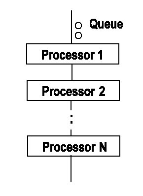
| MULTIPLE PARALLEL PROCESSORS |
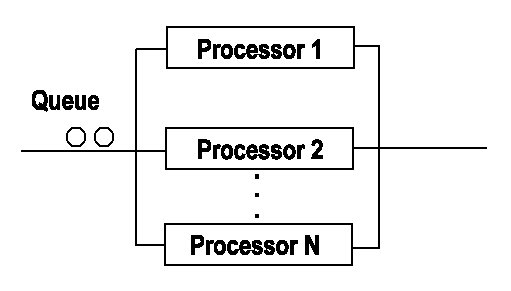 |
| Arrival and Departure Algorithms for Multiple Parallel Processors |
  |
| |
|
| MULTIPLE SERIES PROCESSORS |
| Intermediate Queues |
| |
| Behaves just like multiple single server models where a departure from processor n is an arrival at processor n+1. |
| |
| No intermediate Queues |
 |
| |
| Networks of Queues |
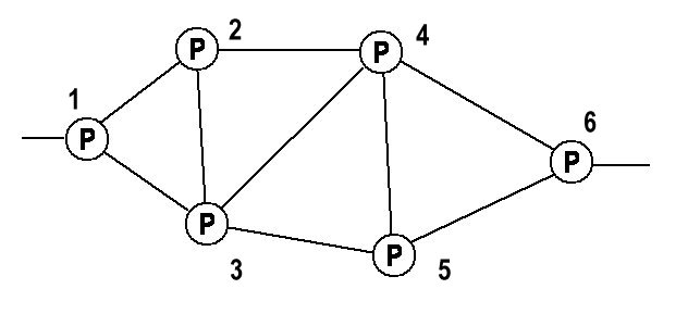 |
| Network Routing Table |
| From/To | 1 | 2 | 3 | 4 | 5 | 6 |
| 1 | - | 2 | 3 | 2 | 3 | 2 |
| 2 | 1 | - | 3 | 4 | 3 | 4 |
| 3 | 1 | 2 | - | 4 | 5 | 5 |
| 4 | 2 | 2 | 3 | - | 5 | 6 |
| 5 | 3 | 3 | 3 | 4 | - | 5 |
| 6 | 5 | 4 | 5 | 4 | 5 | - |
|
| |
|
|
|
| Copyright © 2011 - 2014 Ken Sochats |